what does a standard deviation close to 1 mean

In statistics, a mensurate of variation

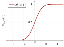
Cumulative probability of a normal distribution with expected value 0 and standard departure 1

In statistics, the standard deviation is a measure of the amount of variation or dispersion of a fix of values.^[1] A low standard divergence indicates that the values tend to be close to the mean (also called the expected value) of the set, while a high standard difference indicates that the values are spread out over a wider range.

Standard deviation may be abbreviated SD, and is most usually represented in mathematical texts and equations by the lower example Greek letter sigma σ, for the population standard deviation, or the Latin letter s, for the sample standard divergence.

The standard deviation of a random variable, sample, statistical population, information set up, or probability distribution is the square root of its variance. It is algebraically simpler, though in practise less robust, than the average absolute deviation.^{[ii] [3]} A useful property of the standard deviation is that, different the variance, information technology is expressed in the same unit as the data.

The standard deviation of a population or sample and the standard error of a statistic (e.g., of the sample mean) are quite different, but related. The sample mean'southward standard fault is the standard deviation of the set of means that would exist plant by cartoon an infinite number of repeated samples from the population and calculating a mean for each sample. The mean's standard error turns out to equal the population standard deviation divided by the square root of the sample size, and is estimated by using the sample standard divergence divided past the square root of the sample size. For case, a poll'south standard error (what is reported equally the margin of error of the poll), is the expected standard deviation of the estimated mean if the same poll were to be conducted multiple times. Thus, the standard mistake estimates the standard departure of an guess, which itself measures how much the gauge depends on the particular sample that was taken from the population.

In science, it is common to study both the standard deviation of the data (as a summary statistic) and the standard error of the approximate (equally a measure of potential error in the findings). Past convention, only effects more than 2 standard errors away from a null expectation are considered "statistically significant", a safeguard against spurious conclusion that is actually due to random sampling error.

When only a sample of data from a population is available, the term standard deviation of the sample or sample standard deviation tin can refer to either the above-mentioned quantity as applied to those data, or to a modified quantity that is an unbiased guess of the population standard deviation (the standard departure of the entire population).

Basic examples [edit]

Population standard difference of grades of 8 students [edit]

Suppose that the entire population of interest is eight students in a particular grade. For a finite ready of numbers, the population standard divergence is found by taking the square root of the average of the squared deviations of the values subtracted from their boilerplate value. The marks of a course of eight students (that is, a statistical population) are the following eight values:

${\displaystyle 2,\ 4,\ 4,\ 4,\ 5,\ v,\ 7,\ 9.}$

These eight data points have the mean (boilerplate) of five:

${\displaystyle \mu ={\frac {2+4+4+4+5+v+7+9}{viii}}={\frac {40}{8}}=v.}$

Get-go, calculate the deviations of each data betoken from the hateful, and square the outcome of each:

${\displaystyle {\brainstorm{array}{lll}(ii-v)^{ii}=(-3)^{two}=nine&&(5-5)^{ii}=0^{2}=0\\(4-five)^{2}=(-one)^{two}=1&&(5-five)^{2}=0^{2}=0\\(4-v)^{2}=(-ane)^{2}=1&&(7-5)^{2}=2^{two}=4\\(four-v)^{ii}=(-1)^{ii}=one&&(nine-5)^{2}=4^{2}=xvi.\\\end{array}}}$

The variance is the mean of these values:

${\displaystyle \sigma ^{2}={\frac {9+i+ane+1+0+0+iv+sixteen}{eight}}={\frac {32}{8}}=4.}$

and the population standard deviation is equal to the foursquare root of the variance:

${\displaystyle \sigma ={\sqrt {4}}=2.}$

This formula is valid just if the eight values with which nosotros began form the complete population. If the values instead were a random sample drawn from some large parent population (for case, they were eight students randomly and independently chosen from a class of 2 one thousand thousand), then one divides past 7 (which is northward − 1) instead of 8 (which is n) in the denominator of the final formula, and the result is ${\textstyle s={\sqrt {32/7}}\approx 2.1.}$ In that case, the effect of the original formula would exist called the sample standard deviation and denoted by s instead of ${\displaystyle \sigma .}$ Dividing by due north − i rather than by n gives an unbiased guess of the variance of the larger parent population. This is known as Bessel's correction.^{[4] [5]} Roughly, the reason for it is that the formula for the sample variance relies on computing differences of observations from the sample hateful, and the sample mean itself was constructed to be equally close as possible to the observations, then only dividing by n would underestimate the variability.

Standard deviation of average height for adult men [edit]

If the population of interest is approximately normally distributed, the standard difference provides information on the proportion of observations above or below sure values. For example, the average summit for adult men in the United States is near lxx inches (177.eight cm), with a standard divergence of around 3 inches (seven.62 cm). This ways that most men (about 68%, bold a normal distribution) have a height within 3 inches (7.62 cm) of the mean (67–73 inches (170.18–185.42 cm)) – one standard divergence – and almost all men (about 95%) have a height within 6 inches (15.24 cm) of the mean (64–76 inches (162.56–193.04 cm)) – two standard deviations. If the standard deviation were zilch, then all men would be exactly lxx inches (177.viii cm) tall. If the standard deviation were 20 inches (l.viii cm), then men would have much more variable heights, with a typical range of nigh 50–ninety inches (127–228.6 cm). Three standard deviations account for 99.seven% of the sample population beingness studied, bold the distribution is normal or bell-shaped (come across the 68–95–99.7 dominion, or the empirical rule, for more information).

Definition of population values [edit]

Let μ be the expected value (the average) of random variable X with density f(x):

$${\displaystyle \mu \equiv \operatorname {E} [X]=\int _{-\infty }^{+\infty }xf(x)\,dx}$$

The standard deviation σ of X is defined equally

$${\displaystyle \sigma \equiv {\sqrt {\operatorname {E} \left[(10-\mu )^{2}\right]}}={\sqrt {\int _{-\infty }^{+\infty }(10-\mu )^{ii}f(ten)\,dx}},}$$

which can be shown to equal ${\textstyle {\sqrt {\operatorname {East} \left[X^{2}\correct]-(\operatorname {East} [Ten])^{ii}}}.}$

Using words, the standard departure is the square root of the variance of X.

The standard divergence of a probability distribution is the same as that of a random variable having that distribution.

Not all random variables have a standard departure. If the distribution has fatty tails going out to infinity, the standard deviation might non exist, because the integral might non converge. The normal distribution has tails going out to infinity, but its mean and standard deviation do exist, considering the tails diminish chop-chop enough. The Pareto distribution with parameter ${\displaystyle \alpha \in (1,2]}$ has a hateful, but not a standard deviation (loosely speaking, the standard deviation is infinite). The Cauchy distribution has neither a hateful nor a standard deviation.

Discrete random variable [edit]

In the case where X takes random values from a finite data ready x _one, x ₂, …, x_{Due north} , with each value having the same probability, the standard deviation is

$${\displaystyle \sigma ={\sqrt {{\frac {one}{Northward}}\left[(x_{1}-\mu )^{2}+(x_{2}-\mu )^{2}+\cdots +(x_{Due north}-\mu )^{two}\right]}},{\text{ where }}\mu ={\frac {one}{N}}(x_{one}+\cdots +x_{Due north}),}$$

or, by using summation annotation,

$${\displaystyle \sigma ={\sqrt {{\frac {ane}{Due north}}\sum _{i=1}^{Northward}(x_{i}-\mu )^{2}}},{\text{ where }}\mu ={\frac {1}{N}}\sum _{i=1}^{North}x_{i}.}$$

If, instead of having equal probabilities, the values have different probabilities, permit x _i have probability p _one, x _two have probability p _two, …, x _N have probability p _Northward . In this case, the standard deviation will be

$${\displaystyle \sigma ={\sqrt {\sum _{i=1}^{North}p_{i}(x_{i}-\mu )^{2}}},{\text{ where }}\mu =\sum _{i=i}^{Due north}p_{i}x_{i}.}$$

Continuous random variable [edit]

The standard difference of a continuous real-valued random variable X with probability density role p(x) is

$${\displaystyle \sigma ={\sqrt {\int _{\mathbf {Ten} }(x-\mu )^{ii}\,p(ten)\,dx}},{\text{ where }}\mu =\int _{\mathbf {Ten} }10\,p(x)\,dx,}$$

and where the integrals are definite integrals taken for ten ranging over the prepare of possible values of the random variableX.

In the case of a parametric family unit of distributions, the standard deviation can be expressed in terms of the parameters. For example, in the case of the log-normal distribution with parameters μ and σ ², the standard deviation is

$${\displaystyle {\sqrt {\left(due east^{\sigma ^{two}}-one\right)e^{2\mu +\sigma ^{ii}}}}.}$$

Estimation [edit]

One can detect the standard departure of an entire population in cases (such as standardized testing) where every fellow member of a population is sampled. In cases where that cannot be done, the standard deviation σ is estimated by examining a random sample taken from the population and computing a statistic of the sample, which is used as an estimate of the population standard deviation. Such a statistic is called an figurer, and the estimator (or the value of the estimator, namely the estimate) is called a sample standard deviation, and is denoted past s (possibly with modifiers).

Unlike in the example of estimating the population mean, for which the sample mean is a elementary calculator with many desirable properties (unbiased, efficient, maximum likelihood), there is no single estimator for the standard deviation with all these properties, and unbiased estimation of standard deviation is a very technically involved problem. Most often, the standard deviation is estimated using the corrected sample standard difference (using N − 1), divers below, and this is ofttimes referred to as the "sample standard deviation", without qualifiers. However, other estimators are better in other respects: the uncorrected figurer (using Due north) yields lower mean squared mistake, while using Northward − 1.5 (for the normal distribution) most completely eliminates bias.

Uncorrected sample standard deviation [edit]

The formula for the population standard deviation (of a finite population) can exist practical to the sample, using the size of the sample as the size of the population (though the bodily population size from which the sample is drawn may be much larger). This calculator, denoted by south _N , is known equally the uncorrected sample standard departure, or sometimes the standard deviation of the sample (considered every bit the unabridged population), and is defined equally follows:^[6]

$${\displaystyle s_{Northward}={\sqrt {{\frac {1}{North}}\sum _{i=one}^{N}\left(x_{i}-{\bar {x}}\right)^{2}}},}$$

where ${\displaystyle \{x_{1},\,x_{2},\,\ldots ,\,x_{N}\}}$ are the observed values of the sample items, and ${\displaystyle {\bar {x}}}$ is the mean value of these observations, while the denominatorN stands for the size of the sample: this is the square root of the sample variance, which is the average of the squared deviations about the sample mean.

This is a consistent computer (it converges in probability to the population value as the number of samples goes to infinity), and is the maximum-likelihood estimate when the population is normally distributed.^{[ citation needed ]} However, this is a biased reckoner, as the estimates are generally too depression. The bias decreases as sample size grows, dropping off as 1/N, and thus is nearly significant for small or moderate sample sizes; for ${\displaystyle N>75}$ the bias is below 1%. Thus for very large sample sizes, the uncorrected sample standard deviation is generally adequate. This estimator also has a uniformly smaller mean squared error than the corrected sample standard deviation.

Corrected sample standard difference [edit]

If the biased sample variance (the second central moment of the sample, which is a downward-biased gauge of the population variance) is used to compute an judge of the population'due south standard deviation, the result is

${\displaystyle s_{Due north}={\sqrt {{\frac {1}{Due north}}\sum _{i=1}^{North}\left(x_{i}-{\bar {x}}\right)^{two}}}.}$

Here taking the square root introduces further downward bias, past Jensen's inequality, due to the foursquare root'due south existence a concave function. The bias in the variance is hands corrected, only the bias from the square root is more than difficult to correct, and depends on the distribution in question.

An unbiased estimator for the variance is given past applying Bessel's correction, using N − 1 instead of North to yield the unbiased sample variance, denoted s ²:

${\displaystyle s^{2}={\frac {1}{N-one}}\sum _{i=1}^{N}\left(x_{i}-{\bar {10}}\correct)^{2}.}$

This figurer is unbiased if the variance exists and the sample values are drawn independently with replacement. N − 1 corresponds to the number of degrees of freedom in the vector of deviations from the mean, ${\displaystyle \textstyle (x_{ane}-{\bar {x}},\;\dots ,\;x_{n}-{\bar {10}}).}$

Taking square roots reintroduces bias (considering the square root is a nonlinear function, which does not commute with the expectation), yielding the corrected sample standard deviation, denoted by south:

${\displaystyle s={\sqrt {{\frac {1}{N-1}}\sum _{i=1}^{N}\left(x_{i}-{\bar {ten}}\correct)^{2}}}.}$

Every bit explained above, while south ² is an unbiased estimator for the population variance, due south is however a biased estimator for the population standard deviation, though markedly less biased than the uncorrected sample standard divergence. This estimator is ordinarily used and generally known but as the "sample standard divergence". The bias may still exist big for small samples (Northward less than x). As sample size increases, the amount of bias decreases. We obtain more information and the difference between ${\displaystyle {\frac {one}{N}}}$ and ${\displaystyle {\frac {ane}{N-one}}}$ becomes smaller.

Unbiased sample standard difference [edit]

For unbiased estimation of standard deviation, there is no formula that works beyond all distributions, different for hateful and variance. Instead, southward is used as a basis, and is scaled past a correction cistron to produce an unbiased estimate. For the normal distribution, an unbiased calculator is given past s/c ₄, where the correction gene (which depends on N) is given in terms of the Gamma part, and equals:

${\displaystyle c_{4}(North)\,=\,{\sqrt {\frac {2}{North-1}}}\,\,\,{\frac {\Gamma \left({\frac {Due north}{2}}\right)}{\Gamma \left({\frac {N-one}{2}}\right)}}.}$

This arises because the sampling distribution of the sample standard deviation follows a (scaled) chi distribution, and the correction factor is the mean of the chi distribution.

An approximation can be given by replacing N − 1 with N − 1.5, yielding:

${\displaystyle {\hat {\sigma }}={\sqrt {{\frac {ane}{N-1.5}}\sum _{i=1}^{North}\left(x_{i}-{\bar {10}}\right)^{ii}}},}$

The mistake in this approximation decays quadratically (as 1/Due north ²), and it is suited for all but the smallest samples or highest precision: for Due north = 3 the bias is equal to 1.iii%, and for N = 9 the bias is already less than 0.one%.

A more than accurate approximation is to supplant ${\displaystyle North-i.5}$ above with ${\displaystyle Due north-1.5+ane/(eight(N-1))}$ .^[7]

For other distributions, the correct formula depends on the distribution, but a dominion of pollex is to use the further refinement of the approximation:

${\displaystyle {\hat {\sigma }}={\sqrt {{\frac {1}{N-1.five-{\frac {1}{iv}}\gamma _{2}}}\sum _{i=1}^{N}\left(x_{i}-{\bar {10}}\right)^{2}}},}$

where γ ₂ denotes the population excess kurtosis. The excess kurtosis may be either known beforehand for certain distributions, or estimated from the data.^[8]

Conviction interval of a sampled standard deviation [edit]

The standard deviation we obtain by sampling a distribution is itself not absolutely accurate, both for mathematical reasons (explained hither by the confidence interval) and for practical reasons of measurement (measurement error). The mathematical result can be described past the confidence interval or CI.

To show how a larger sample will make the conviction interval narrower, consider the post-obit examples: A small population of Due north = two has only 1 degree of freedom for estimating the standard deviation. The result is that a 95% CI of the SD runs from 0.45 × SD to 31.nine × SD; the factors here are as follows:

${\displaystyle \Pr \left(q_{\frac {\blastoff }{2}}<g{\frac {s^{2}}{\sigma ^{2}}}<q_{ane-{\frac {\alpha }{2}}}\right)=1-\alpha ,}$

where ${\displaystyle q_{p}}$ is the p-th quantile of the chi-square distribution with k degrees of freedom, and ${\displaystyle ane-\alpha }$ is the confidence level. This is equivalent to the following:

${\displaystyle \Pr \left(k{\frac {south^{2}}{q_{1-{\frac {\alpha }{2}}}}}<\sigma ^{2}<thou{\frac {s^{ii}}{q_{\frac {\alpha }{2}}}}\correct)=1-\alpha .}$

With k = 1, ${\displaystyle q_{0.025}=0.000982}$ and ${\displaystyle q_{0.975}=5.024}$ . The reciprocals of the foursquare roots of these ii numbers give united states of america the factors 0.45 and 31.9 given in a higher place.

A larger population of N = x has 9 degrees of freedom for estimating the standard deviation. The same computations every bit higher up give united states in this instance a 95% CI running from 0.69 × SD to ane.83 × SD. Then fifty-fifty with a sample population of 10, the actual SD can however be nearly a cistron ii higher than the sampled SD. For a sample population N=100, this is downward to 0.88 × SD to ane.16 × SD. To be more than sure that the sampled SD is shut to the actual SD we need to sample a large number of points.

These same formulae tin can be used to obtain confidence intervals on the variance of residuals from a to the lowest degree squares fit under standard normal theory, where k is at present the number of degrees of liberty for error.

Bounds on standard deviation [edit]

For a prepare of N > iv data spanning a range of values R, an upper spring on the standard divergence southward is given past s = 0.6R.^[9] An gauge of the standard deviation for N > 100 data taken to be approximately normal follows from the heuristic that 95% of the expanse under the normal bend lies roughly ii standard deviations to either side of the hateful, and then that, with 95% probability the total range of values R represents four standard deviations so that due south ≈ R/four. This and so-called range dominion is useful in sample size interpretation, as the range of possible values is easier to estimate than the standard deviation. Other divisors K(Due north) of the range such that s ≈ R/Thousand(N) are available for other values of N and for non-normal distributions.^[10]

Identities and mathematical backdrop [edit]

The standard difference is invariant under changes in location, and scales directly with the scale of the random variable. Thus, for a abiding c and random variables Ten and Y:

${\displaystyle {\begin{aligned}\sigma (c)&=0\\\sigma (10+c)&=\sigma (X),\\\sigma (cX)&=|c|\sigma (X).\finish{aligned}}}$

The standard deviation of the sum of two random variables can be related to their individual standard deviations and the covariance between them:

${\displaystyle \sigma (X+Y)={\sqrt {\operatorname {var} (X)+\operatorname {var} (Y)+ii\,\operatorname {cov} (X,Y)}}.\,}$

where ${\displaystyle \textstyle \operatorname {var} \,=\,\sigma ^{two}}$ and ${\displaystyle \textstyle \operatorname {cov} }$ stand up for variance and covariance, respectively.

The calculation of the sum of squared deviations can be related to moments calculated direct from the data. In the post-obit formula, the letter E is interpreted to mean expected value, i.e., mean.

${\displaystyle \sigma (X)={\sqrt {\operatorname {East} \left[(X-\operatorname {East} [Ten])^{2}\correct]}}={\sqrt {\operatorname {E} \left[X^{2}\correct]-(\operatorname {E} [X])^{2}}}.}$

The sample standard deviation tin can be computed as:

${\displaystyle s(X)={\sqrt {\frac {North}{N-i}}}{\sqrt {\operatorname {Due east} \left[(Ten-\operatorname {E} [X])^{2}\right]}}.}$

For a finite population with equal probabilities at all points, we accept

${\displaystyle {\sqrt {{\frac {one}{N}}\sum _{i=1}^{Northward}\left(x_{i}-{\bar {ten}}\right)^{2}}}={\sqrt {{\frac {one}{Northward}}\left(\sum _{i=1}^{Northward}x_{i}^{2}\right)-{\bar {x}}^{2}}}={\sqrt {\left({\frac {i}{N}}\sum _{i=1}^{N}x_{i}^{2}\right)-\left({\frac {one}{North}}\sum _{i=1}^{N}x_{i}\correct)^{2}}},}$

which means that the standard deviation is equal to the square root of the difference betwixt the average of the squares of the values and the square of the average value.

See computational formula for the variance for proof, and for an analogous result for the sample standard deviation.

Estimation and application [edit]

Example of samples from two populations with the same mean just unlike standard deviations. Scarlet population has mean 100 and SD 10; blue population has mean 100 and SD 50.

A big standard deviation indicates that the data points can spread far from the mean and a small standard deviation indicates that they are clustered closely effectually the mean.

For example, each of the three populations {0, 0, 14, 14}, {0, 6, 8, xiv} and {6, 6, 8, 8} has a mean of 7. Their standard deviations are 7, 5, and 1, respectively. The 3rd population has a much smaller standard deviation than the other two because its values are all close to 7. These standard deviations have the same units as the data points themselves. If, for example, the information set {0, vi, 8, fourteen} represents the ages of a population of four siblings in years, the standard deviation is v years. As some other case, the population {grand, 1006, 1008, 1014} may represent the distances traveled by four athletes, measured in meters. It has a hateful of 1007 meters, and a standard deviation of v meters.

Standard deviation may serve as a measure of dubiety. In physical scientific discipline, for example, the reported standard deviation of a group of repeated measurements gives the precision of those measurements. When deciding whether measurements concur with a theoretical prediction, the standard difference of those measurements is of crucial importance: if the mean of the measurements is too far away from the prediction (with the distance measured in standard deviations), so the theory existence tested probably needs to be revised. This makes sense since they autumn outside the range of values that could reasonably be expected to occur, if the prediction were correct and the standard deviation accordingly quantified. See prediction interval.

While the standard divergence does measure out how far typical values tend to exist from the mean, other measures are available. An case is the mean absolute deviation, which might be considered a more than direct measure of boilerplate distance, compared to the root mean square distance inherent in the standard difference.

Awarding examples [edit]

The practical value of understanding the standard difference of a fix of values is in affectionate how much variation there is from the boilerplate (mean).

Experiment, industrial and hypothesis testing [edit]

Standard departure is ofttimes used to compare real-world information against a model to test the model. For example, in industrial applications the weight of products coming off a production line may need to comply with a legally required value. Past weighing some fraction of the products an boilerplate weight can exist found, which will always exist slightly dissimilar from the long-term boilerplate. By using standard deviations, a minimum and maximum value can exist calculated that the averaged weight will exist within some very high percentage of the time (99.9% or more than). If information technology falls outside the range then the production process may need to be corrected. Statistical tests such equally these are specially important when the testing is relatively expensive. For example, if the production needs to be opened and drained and weighed, or if the production was otherwise used upward by the examination.

In experimental science, a theoretical model of reality is used. Particle physics conventionally uses a standard of "5 sigma" for the declaration of a discovery. A five-sigma level translates to 1 chance in 3.5 million that a random fluctuation would yield the result. This level of certainty was required in order to assert that a particle consistent with the Higgs boson had been discovered in two independent experiments at CERN,^[eleven] also leading to the proclamation of the first observation of gravitational waves,^[12] and confirmation of global warming.^[13]

Weather [edit]

As a simple case, consider the average daily maximum temperatures for two cities, ane inland and one on the coast. Information technology is helpful to sympathize that the range of daily maximum temperatures for cities well-nigh the coast is smaller than for cities inland. Thus, while these two cities may each have the same average maximum temperature, the standard departure of the daily maximum temperature for the coastal metropolis volition be less than that of the inland city every bit, on whatsoever detail day, the actual maximum temperature is more likely to exist farther from the boilerplate maximum temperature for the inland city than for the coastal i.

Finance [edit]

In finance, standard deviation is oftentimes used as a measure of the hazard associated with price-fluctuations of a given nugget (stocks, bonds, property, etc.), or the risk of a portfolio of assets^[14] (actively managed mutual funds, alphabetize mutual funds, or ETFs). Take chances is an important cistron in determining how to efficiently manage a portfolio of investments because it determines the variation in returns on the asset and/or portfolio and gives investors a mathematical ground for investment decisions (known as mean-variance optimization). The cardinal concept of risk is that as it increases, the expected return on an investment should increase too, an increment known as the gamble premium. In other words, investors should look a higher return on an investment when that investment carries a higher level of chance or uncertainty. When evaluating investments, investors should judge both the expected return and the uncertainty of future returns. Standard deviation provides a quantified estimate of the uncertainty of futurity returns.

For example, assume an investor had to choose betwixt 2 stocks. Stock A over the past 20 years had an average return of ten percent, with a standard deviation of 20 percentage points (pp) and Stock B, over the same menses, had boilerplate returns of 12 per centum but a college standard deviation of 30 pp. On the basis of chance and return, an investor may determine that Stock A is the safer choice, because Stock B's additional two percentage points of return is not worth the boosted 10 pp standard deviation (greater risk or uncertainty of the expected return). Stock B is likely to fall brusque of the initial investment (but also to exceed the initial investment) more often than Stock A under the same circumstances, and is estimated to return but two percent more than on boilerplate. In this example, Stock A is expected to earn about 10 percentage, plus or minus 20 pp (a range of thirty percent to −10 percentage), well-nigh two-thirds of the futurity twelvemonth returns. When considering more farthermost possible returns or outcomes in hereafter, an investor should expect results of as much equally 10 per centum plus or minus 60 pp, or a range from 70 per centum to −50 percent, which includes outcomes for 3 standard deviations from the average render (about 99.seven percent of likely returns).

Calculating the average (or arithmetic mean) of the render of a security over a given period will generate the expected return of the asset. For each menstruum, subtracting the expected return from the actual return results in the divergence from the hateful. Squaring the difference in each menstruum and taking the average gives the overall variance of the return of the asset. The larger the variance, the greater take chances the security carries. Finding the square root of this variance will give the standard deviation of the investment tool in question.

Population standard deviation is used to prepare the width of Bollinger Bands, a technical analysis tool. For example, the upper Bollinger Band is given equally ${\displaystyle \textstyle {\bar {x}}+n\sigma _{x}.}$ The most commonly used value for due north is ii; there is almost a five percent take chances of going exterior, assuming a normal distribution of returns.

Financial fourth dimension series are known to exist not-stationary series, whereas the statistical calculations above, such as standard deviation, utilize only to stationary serial. To apply the in a higher place statistical tools to not-stationary serial, the series first must be transformed to a stationary serial, enabling use of statistical tools that now have a valid basis from which to work.

Geometric interpretation [edit]

To proceeds some geometric insights and clarification, we will start with a population of three values, x ₁, x ₂, x _three. This defines a point P = (ten ₁, x _ii, ten ₃) in R ³. Consider the line L = {(r, r, r) : r ∈ R}. This is the "main diagonal" going through the origin. If our three given values were all equal, then the standard deviation would be zero and P would lie on L. And so it is not unreasonable to presume that the standard deviation is related to the distance of P to L. That is indeed the example. To move orthogonally from L to the indicate P, one begins at the indicate:

${\displaystyle Thou=\left({\bar {ten}},{\bar {x}},{\bar {x}}\right)}$

whose coordinates are the mean of the values nosotros started out with.

Derivation of ${\displaystyle 1000=\left({\bar {ten}},{\bar {x}},{\bar {ten}}\right)}$

${\displaystyle M}$ is on ${\displaystyle Fifty}$ therefore ${\displaystyle M=(\ell ,\ell ,\ell )}$ for some ${\displaystyle \ell \in \mathbb {R} }$ . The line ${\displaystyle L}$ is to be orthogonal to the vector from ${\displaystyle M}$ to ${\displaystyle P}$ . Therefore: ${\displaystyle {\begin{aligned}L\cdot (P-M)&=0\\[4pt](r,r,r)\cdot (x_{1}-\ell ,x_{two}-\ell ,x_{3}-\ell )&=0\\[4pt]r(x_{1}-\ell +x_{2}-\ell +x_{iii}-\ell )&=0\\[4pt]r\left(\sum _{i}x_{i}-3\ell \right)&=0\\[4pt]\sum _{i}x_{i}-3\ell &=0\\[4pt]{\frac {i}{3}}\sum _{i}x_{i}&=\ell \\[4pt]{\bar {x}}&=\ell \terminate{aligned}}}$

A fiddling algebra shows that the distance betwixt P and M (which is the same as the orthogonal distance between P and the line 50) ${\textstyle {\sqrt {\sum _{i}\left(x_{i}-{\bar {x}}\correct)^{2}}}}$ is equal to the standard deviation of the vector (x ₁, ten ₂, x ₃), multiplied by the square root of the number of dimensions of the vector (3 in this case).

Chebyshev's inequality [edit]

An observation is rarely more than a few standard deviations away from the mean. Chebyshev's inequality ensures that, for all distributions for which the standard deviation is defined, the corporeality of data inside a number of standard deviations of the mean is at least as much as given in the following table.

Distance from hateful	Minimum population
${\displaystyle {\sqrt {two}}\,\sigma }$	50%
twoσ	75%
3σ	89%
ivσ	94%
5σ	96%
half-dozenσ	97%
${\displaystyle grand\sigma }$	${\displaystyle 1-{\frac {1}{1000^{two}}}}$ [15]
${\displaystyle {\frac {1}{\sqrt {one-\ell }}}\,\sigma }$	${\displaystyle \ell }$

Rules for normally distributed data [edit]

Nighttime blueish is one standard divergence on either side of the mean. For the normal distribution, this accounts for 68.27 percent of the prepare; while 2 standard deviations from the mean (medium and dark blue) account for 95.45 percent; 3 standard deviations (calorie-free, medium, and nighttime blue) account for 99.73 percent; and four standard deviations account for 99.994 percent. The two points of the bend that are one standard divergence from the mean are likewise the inflection points.

The key limit theorem states that the distribution of an boilerplate of many contained, identically distributed random variables tends toward the famous bell-shaped normal distribution with a probability density function of

${\displaystyle f\left(x,\mu ,\sigma ^{2}\right)={\frac {1}{\sigma {\sqrt {2\pi }}}}e^{-{\frac {i}{2}}\left({\frac {x-\mu }{\sigma }}\right)^{2}}}$

where μ is the expected value of the random variables, σ equals their distribution'southward standard departure divided by north ^1/ii, and due north is the number of random variables. The standard deviation therefore is simply a scaling variable that adjusts how broad the curve will be, though information technology as well appears in the normalizing abiding.

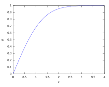
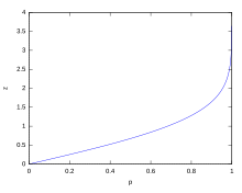
If a data distribution is approximately normal, then the proportion of data values within z standard deviations of the mean is defined by:

${\displaystyle {\text{Proportion}}=\operatorname {erf} \left({\frac {z}{\sqrt {2}}}\right)}$

where ${\displaystyle \textstyle \operatorname {erf} }$ is the fault function. The proportion that is less than or equal to a number, 10, is given by the cumulative distribution function:

${\displaystyle {\text{Proportion}}\leq x={\frac {one}{2}}\left[1+\operatorname {erf} \left({\frac {10-\mu }{\sigma {\sqrt {2}}}}\correct)\right]={\frac {1}{two}}\left[1+\operatorname {erf} \left({\frac {z}{\sqrt {2}}}\correct)\right]}$ .^[sixteen]

If a data distribution is approximately normal then about 68 percent of the data values are within one standard deviation of the hateful (mathematically, μ ±σ, where μ is the arithmetic mean), about 95 percent are within ii standard deviations (μ ± iiσ), and about 99.vii percent prevarication inside three standard deviations (μ ± 3σ). This is known as the 68–95–99.7 rule, or the empirical rule.

For diverse values of z, the pct of values expected to prevarication in and outside the symmetric interval, CI = (−zσ,zσ), are as follows:

Confidence interval	Proportion within	Proportion without
	Percentage	Percentage	Fraction
0.318639 σ	25%	75%	3 / 4
0.674490 σ	50%	50%	1 / 2
0.977925 σ	66.6667%	33.3333%	1 / 3
0.994458 σ	68%	32%	1 / iii.125
1σ	68.2689492 %	31.7310508 %	1 / 3.1514872
1.281552 σ	80%	20%	1 / 5
one.644854 σ	90%	ten%	ane / 10
one.959964 σ	95%	v%	1 / 20
2σ	95.4499736 %	four.5500264 %	1 / 21.977895
two.575829 σ	99%	1%	one / 100
3σ	99.7300204 %	0.2699796 %	1 / 370.398
iii.290527 σ	99.9%	0.1%	1 / one thousand
3.890592 σ	99.99%	0.01%	1 / ten000
4σ	99.993666 %	0.006334 %	ane / xv787
four.417173 σ	99.999%	0.001%	1 / 100000
4.v σ	99.999320 465 3751%	0.000679 534 6249%	1 / 147159.5358 6.8 / 1000 000
iv.891638 σ	99.9999%	0.0001%	1 / i000 000
vσ	99.999942 6697 %	0.000057 3303 %	ane / i744 278
five.326724 σ	99.99999 %	0.00001 %	1 / x000 000
v.730729 σ	99.999999 %	0.000001 %	1 / 100000 000
6 σ	99.999999 8027 %	0.000000 1973 %	1 / 506797 346
6.109410 σ	99.9999999 %	0.0000001 %	1 / one000 000 000
half dozen.466951 σ	99.999999 99 %	0.000000 01 %	1 / 10000 000 000
6.806502 σ	99.999999 999 %	0.000000 001 %	1 / 100000 000 000
sevenσ	99.999999 999 7440%	0.000000 000 256 %	1 / 390682 215 445

Relationship between standard departure and mean [edit]

The mean and the standard deviation of a set of data are descriptive statistics usually reported together. In a certain sense, the standard deviation is a "natural" measure of statistical dispersion if the center of the information is measured almost the mean. This is because the standard deviation from the mean is smaller than from any other point. The precise statement is the following: suppose x _one, ..., x _n are existent numbers and define the function:

${\displaystyle \sigma (r)={\sqrt {{\frac {1}{N-1}}\sum _{i=1}^{Due north}\left(x_{i}-r\correct)^{two}}}.}$

Using calculus or past completing the square, it is possible to bear witness that σ(r) has a unique minimum at the mean:

${\displaystyle r={\bar {x}}.\,}$

Variability can too be measured by the coefficient of variation, which is the ratio of the standard difference to the mean. It is a dimensionless number.

Standard deviation of the mean [edit]

Often, we want some information about the precision of the mean we obtained. We can obtain this past determining the standard difference of the sampled hateful. Assuming statistical independence of the values in the sample, the standard deviation of the mean is related to the standard deviation of the distribution past:

${\displaystyle \sigma _{\text{mean}}={\frac {1}{\sqrt {N}}}\sigma }$

where N is the number of observations in the sample used to estimate the mean. This tin can easily be proven with (see basic backdrop of the variance):

${\displaystyle {\brainstorm{aligned}\operatorname {var} (X)&\equiv \sigma _{Ten}^{2}\\\operatorname {var} (X_{1}+X_{2})&\equiv \operatorname {var} (X_{one})+\operatorname {var} (X_{2})\\\end{aligned}}}$

(Statistical independence is assumed.)

${\displaystyle \operatorname {var} (cX_{one})\equiv c^{2}\,\operatorname {var} (X_{1})}$

hence

${\displaystyle {\begin{aligned}\operatorname {var} ({\text{mean}})&=\operatorname {var} \left({\frac {1}{N}}\sum _{i=one}^{N}X_{i}\right)={\frac {1}{Due north^{two}}}\operatorname {var} \left(\sum _{i=1}^{Northward}X_{i}\correct)\\&={\frac {ane}{N^{ii}}}\sum _{i=ane}^{North}\operatorname {var} (X_{i})={\frac {N}{N^{2}}}\operatorname {var} (X)={\frac {1}{N}}\operatorname {var} (Ten).\end{aligned}}}$

Resulting in:

${\displaystyle \sigma _{\text{mean}}={\frac {\sigma }{\sqrt {N}}}.}$

In guild to guess the standard deviation of the mean ${\displaystyle \sigma _{\text{mean}}}$ it is necessary to know the standard deviation of the unabridged population ${\displaystyle \sigma }$ beforehand. All the same, in most applications this parameter is unknown. For example, if a series of 10 measurements of a previously unknown quantity is performed in a laboratory, it is possible to calculate the resulting sample mean and sample standard deviation, just information technology is impossible to calculate the standard deviation of the mean.

Rapid calculation methods [edit]

The following 2 formulas can stand for a running (repeatedly updated) standard deviation. A set of 2 power sums s ₁ and s ₂ are computed over a set up of N values of ten, denoted every bit x _i, ..., x _N :

${\displaystyle s_{j}=\sum _{one thousand=one}^{North}{x_{one thousand}^{j}}.}$

Given the results of these running summations, the values Due north, s ₁, s ₂ can be used at whatever time to compute the current value of the running standard deviation:

${\displaystyle \sigma ={\frac {\sqrt {Ns_{ii}-s_{1}^{2}}}{N}}}$

Where North, as mentioned above, is the size of the set of values (or can too be regarded every bit due south ₀).

Similarly for sample standard departure,

${\displaystyle s={\sqrt {\frac {Ns_{2}-s_{ane}^{2}}{N(Northward-1)}}}.}$

In a computer implementation, equally the 2 due south _j sums become big, nosotros need to consider round-off error, arithmetic overflow, and arithmetic underflow. The method below calculates the running sums method with reduced rounding errors.^[17] This is a "ane pass" algorithm for computing variance of n samples without the demand to store prior information during the adding. Applying this method to a time series volition outcome in successive values of standard difference corresponding to n information points equally n grows larger with each new sample, rather than a abiding-width sliding window calculation.

For k = 1, ..., n:

${\displaystyle {\brainstorm{aligned}A_{0}&=0\\A_{k}&=A_{g-1}+{\frac {x_{k}-A_{k-1}}{k}}\stop{aligned}}}$

where A is the mean value.

${\displaystyle {\begin{aligned}Q_{0}&=0\\Q_{k}&=Q_{k-1}+{\frac {k-one}{k}}\left(x_{k}-A_{k-one}\right)^{ii}=Q_{k-one}+\left(x_{thousand}-A_{k-1}\right)\left(x_{grand}-A_{k}\right)\terminate{aligned}}}$

Note: ${\displaystyle Q_{1}=0}$ since ${\displaystyle grand-one=0}$ or ${\displaystyle x_{1}=A_{1}}$

Sample variance:

${\displaystyle s_{n}^{ii}={\frac {Q_{north}}{n-one}}}$

Population variance:

${\displaystyle \sigma _{n}^{2}={\frac {Q_{n}}{n}}}$

Weighted calculation [edit]

When the values x_i are weighted with unequal weights w_i , the ability sums southward ₀, south _one, s _ii are each computed as:

${\displaystyle s_{j}=\sum _{k=1}^{Northward}w_{k}x_{1000}^{j}.\,}$

And the standard difference equations remain unchanged. due south ₀ is at present the sum of the weights and not the number of samples Due north.

The incremental method with reduced rounding errors can too exist applied, with some additional complication.

A running sum of weights must be computed for each k from one to north:

${\displaystyle {\begin{aligned}W_{0}&=0\\W_{k}&=W_{k-1}+w_{m}\end{aligned}}}$

and places where ane/n is used above must be replaced by due west_i /W_northward :

${\displaystyle {\begin{aligned}A_{0}&=0\\A_{k}&=A_{k-1}+{\frac {w_{k}}{W_{k}}}\left(x_{one thousand}-A_{k-ane}\right)\\Q_{0}&=0\\Q_{k}&=Q_{thou-1}+{\frac {w_{thousand}W_{thou-i}}{W_{k}}}\left(x_{k}-A_{1000-1}\correct)^{2}=Q_{yard-1}+w_{k}\left(x_{k}-A_{k-1}\right)\left(x_{m}-A_{k}\right)\end{aligned}}}$

In the final division,

${\displaystyle \sigma _{n}^{ii}={\frac {Q_{north}}{W_{due north}}}\,}$

and

${\displaystyle s_{due north}^{ii}={\frac {Q_{n}}{W_{n}-one}},}$

or

${\displaystyle s_{n}^{2}={\frac {n'}{n'-1}}\sigma _{n}^{2},}$

where n is the total number of elements, and n' is the number of elements with non-zero weights.

The above formulas become equal to the simpler formulas given above if weights are taken as equal to one.

History [edit]

The term standard deviation was first used in writing by Karl Pearson in 1894, following his use of it in lectures.^{[18] [nineteen]} This was equally a replacement for earlier culling names for the aforementioned idea: for example, Gauss used hateful error.^[twenty]

College dimensions [edit]

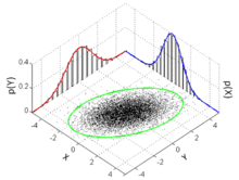
The standard deviation ellipse (light-green) of a two-dimensional normal distribution

In 2 dimensions, the standard deviation tin can be illustrated with the standard departure ellipse (see Multivariate normal distribution § Geometric interpretation).

See also [edit]

• 68–95–99.seven rule
• Accuracy and precision
• Chebyshev's inequality An inequality on location and calibration parameters
• Coefficient of variation
• Cumulant
• Deviation (statistics)
• Distance correlation Distance standard difference
• Error bar
• Geometric standard deviation
• Mahalanobis altitude generalizing number of standard deviations to the mean
• Mean absolute error
• Pooled variance
• Propagation of dubiousness
• Percentile
• Raw information
• Robust standard deviation
• Root mean square
• Sample size
• Samuelson'southward inequality
• Six Sigma
• Standard error
• Standard score
• Yamartino method for calculating standard divergence of current of air direction

References [edit]

1. ^ Bland, J.M.; Altman, D.G. (1996). "Statistics notes: measurement error". BMJ. 312 (7047): 1654. doi:x.1136/bmj.312.7047.1654. PMC2351401. PMID 8664723.
2. ^ Gauss, Carl Friedrich (1816). "Bestimmung der Genauigkeit der Beobachtungen". Zeitschrift für Astronomie und Verwandte Wissenschaften. 1: 187–197.
3. ^ Walker, Helen (1931). Studies in the History of the Statistical Method. Baltimore, Dr.: Williams & Wilkins Co. pp. 24–25.
4. ^ Weisstein, Eric W. "Bessel'south Correction". MathWorld.
5. ^ "Standard Divergence Formulas". www.mathsisfun.com . Retrieved 21 Baronial 2020.
6. ^ Weisstein, Eric W. "Standard Divergence". mathworld.wolfram.com . Retrieved 21 August 2020.
7. ^ Gurland, John; Tripathi, Ram C. (1971), "A Simple Approximation for Unbiased Estimation of the Standard Deviation", The American Statistician, 25 (4): 30–32, doi:10.2307/2682923, JSTOR 2682923
8. ^ "Standard Divergence Calculator". PureCalculators. 11 July 2021. Retrieved 14 September 2021.
9. ^ Shiffler, Ronald E.; Harsha, Phillip D. (1980). "Upper and Lower Bounds for the Sample Standard Departure". Didactics Statistics. 2 (iii): 84–86. doi:x.1111/j.1467-9639.1980.tb00398.x.
10. ^ Browne, Richard H. (2001). "Using the Sample Range as a Ground for Calculating Sample Size in Power Calculations". The American Statistician. 55 (4): 293–298. doi:10.1198/000313001753272420. JSTOR 2685690. S2CID 122328846.
11. ^ "CERN experiments observe particle consequent with long-sought Higgs boson | CERN press role". Printing.web.cern.ch. 4 July 2012. Archived from the original on 25 March 2016. Retrieved thirty May 2015.
12. ^ LIGO Scientific Collaboration, Virgo Collaboration (2016), "Observation of Gravitational Waves from a Binary Black Hole Merger", Physical Review Letters, 116 (6): 061102, arXiv:1602.03837, Bibcode:2016PhRvL.116f1102A, doi:x.1103/PhysRevLett.116.061102, PMID 26918975, S2CID 124959784
13. ^ Alister Doyle (25 Feb 2019). "Evidence for human being-made global warming hits 'gilded standard': scientists". Reuters . Retrieved 23 March 2021.
14. ^ "What is Standard Deviation". Pristine. Retrieved 29 October 2011.
15. ^ Ghahramani, Saeed (2000). Fundamentals of Probability (2nd ed.). New Jersey: Prentice Hall. p. 438.
16. ^ Eric Due west. Weisstein. "Distribution Office". MathWorld—A Wolfram Spider web Resource. Retrieved 30 September 2014.
17. ^ Welford, BP (August 1962). "Note on a Method for Computing Corrected Sums of Squares and Products". Technometrics. 4 (3): 419–420. CiteSeerXx.1.1.302.7503. doi:10.1080/00401706.1962.10490022.
18. ^ Dodge, Yadolah (2003). The Oxford Dictionary of Statistical Terms . Oxford Academy Press. ISBN978-0-19-920613-1.
19. ^ Pearson, Karl (1894). "On the autopsy of asymmetrical frequency curves". Philosophical Transactions of the Royal Society A. 185: 71–110. Bibcode:1894RSPTA.185...71P. doi:10.1098/rsta.1894.0003.
20. ^ Miller, Jeff. "Earliest Known Uses of Some of the Words of Mathematics".

External links [edit]

• "Quadratic deviation", Encyclopedia of Mathematics, Ems Press, 2001 [1994]
• "Standard Difference Computer"

foxfeavainnince.blogspot.com

Source: https://en.wikipedia.org/wiki/Standard_deviation

Share this post